(GPCE 2022) A modern Point of View of programming in Image Processing

In this document we provide additional example illustrating the relevance of using image views in image processing algorithms.

Alphablending

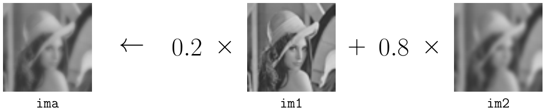
The alphablending algorithm consists in blending two images together, with weight factors, into a resulting image.

For instance, here is how one would write the alphablending algorithm with naive C code:

void blend_inplace(const uint8_t* ima1, uint8_t* ima2, float alpha,
                   int width, int height, int stride1, int stride2) {
  for (int y = 0; y < height; ++y) {
    const uint8_t* iptr = ima1 + y * stride1;
    uint8_t* optr = ima2 + y * stride2;
    for (int x = 0; x < width; ++x)
      optr[x] = iptr[x] * alpha + optr[x] * (1-alpha);
  }
}

This version does not scale. If the practitioner wants to restrict his images with a mask, or a ROI, he needs to use other overloads of the algorithm where this option is offered:

void blend_inplace(const uint8_t* ima1, uint8_t* ima2, const uint8_t* mask, float alpha,
                   int width, int height, int stride1, int stride2);
void blend_inplace(const uint8_t* ima1, uint8_t* ima2, const point2d& roi_tl, const point2d& roi_br,
                   float alpha, int width, int height, int stride1, int stride2);
void blend_inplace(const uint8_t* ima1, uint8_t* ima2, const uint8_t* mask, const point2d& roi_tl,
                   const point2d& roi_br, float alpha, int width, int height, int stride1, int stride2);

If the practitioner wants to restrict the color channel and only process the red or blue channel, then other overloads will be necessary. And the cardinality explode with each option we want to support on the algorithm.

With image views, writing the alphablending algorithm becomes as simple as writing the following code:

auto alphablend = [](auto ima1, auto ima2, float alpha) {
        return alpha * ima1 + (1 - alpha) * ima2;
};

And using it is equivalent to write :

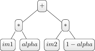
This view does not do the computation unless the value of a pixel is explicitly requested. Instead, it builds an Abstract Syntax Tree (AST) representing the chained computation necessary in order to get the value of a pixel. The AST of the alphablending view is shown:

This way, as the new alphablend algorithm accept as input an image and in our design, an image is a view then we do not need to multiply the number of overload for an algorithm. Instead, we can just chain views before feeding our restricted images to the algorithm:

auto ima = alphablend(ima1, ima2, 0.2); // User-defined view
auto ima_roi = alphablend(view::clip(ima1, roi), view::clip(ima2, roi), 0.2); // ROI
auto ima_mask = alphablend(view::mask(ima1, mask), view::mask(ima2, mask), 0.2); // Mask
auto ima_mask_roi = alphablend(view::clip(iew::mask(ima1, mask), roi),
                               view::clip(view::mask(ima2, mask), roi), 0.2); // Mask + ROI
auto ima_red = alphablend(view::red(ima1), view::red(ima2), 0.2); // Red channel

Connected-component labeling

A common operation in Image processing is to label connected-component in an image in order to get information about those regions, or to perform operation on those regions (coloring, extraction, etc.). Let us suppose that we are able to generate load an image and its connected-component labeled counterpart thanks to state-of-the-art algorithm. We would be able to get:

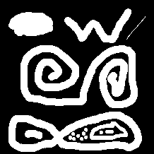
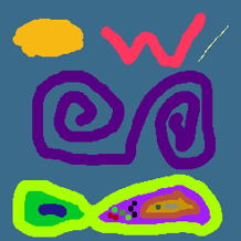
Now it is possible to compute stats on those labels, and to use stats to perform operations directly. This example set to the color red to all region whose number of connected components is superior or equal to 600 and inferior to 4500.

This example also illustrate the usage of the zip view, which is the functional programming construct to assemble several images into one whose value is a tuple of the original values of the underlying images.

// Decorate image to add label attribute to pixel
// colored_ouput is a copy of input transposed into a rgb8 image
auto ima_labelized = view::zip(colored_output, ima_labels);

// Compute stats such as number of connected component by label
// map<int, unsigned> : label -> nb
auto nb_conn_comps = compute_nb_connected_components(ima_labels);

// filter labelized by number of connected component
auto min_comps    = 600u;
auto max_comps    = 4500u;
auto ima_filtered = view::filter(ima_labelized, [&](auto v) {
  auto&& [val, lab] = v;
  return label_count[lab] > min_comps && label_count[lab] < max_comps;
});

// fill those areas in red
auto red = rgb8{255, 0, 0};
fill(ima_filtered, std::make_tuple(red, 0u));

This will output the following image:

Workload showing view performance improvement

This supplementary material includes source code (in the snippets directory) showing performance improvement of views on a simple workload. This workload is illustrated in the following figure:

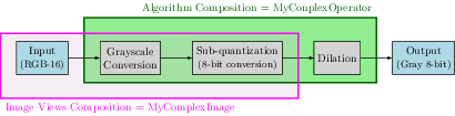
The experiment benchmarks one pipeline running 3 algorithms (to_gray, sub-quantization and dilation) one after the other, whereas the other pipeline compose the two first algorithms (to_gray, sub-quantization) into an image view, to then feed it to the dilation algorithm.

The performance boost of using views is about 20% (133 vs 106ms) on a 20MPix RGB16 images (i7-2600 CPU @ 3.40GHz, single-threaded). The dilation is done with a small 3x3 square structuring element using tiling for caching input values.