Difference between revisions of "Publications/xu.15.prl.inc"
From LRDE
Yongchao Xu (talk | contribs) |
Yongchao Xu (talk | contribs) |
||
| (45 intermediate revisions by the same user not shown) | |||
| Line 1: | Line 1: | ||
== Materials == |
== Materials == |
||
| − | === Mumford-Shah Simplification on the |
+ | === Mumford-Shah Simplification on the Color Tree of Shapes === |
You can download the x86_64 binary to compute the Mumford-Shah simplification running |
You can download the x86_64 binary to compute the Mumford-Shah simplification running |
||
on the color tree of shapes [https://lrde.epita.fr/~xu/bin/mumford_shah_on_ctos Here]. |
on the color tree of shapes [https://lrde.epita.fr/~xu/bin/mumford_shah_on_ctos Here]. |
||
| Line 16: | Line 16: | ||
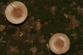
File:carlinet.15.tip-nopeeking.png|Input RGB Image |
File:carlinet.15.tip-nopeeking.png|Input RGB Image |
||
File:carlinet.15.tip-nopeeking_simp.png|Output Simplified Image |
File:carlinet.15.tip-nopeeking_simp.png|Output Simplified Image |
||
| + | File:xu.15.prl-kata.png|Input RGB Image |
||
| + | File:xu.15.prl-kata_simp.png|Output Simplified Image |
||
</gallery> |
</gallery> |
||
| + | === Saliency Map Computation Relying on Mumford-Shah-Salient Level Line Selection === |
||
| − | === Multivariate Tree of Shapes Computation Binaries === |
||
| + | You can download the x86_64 binary to compute the saliency map representing hierarchical image simplification and segmentation [https://lrde.epita.fr/~xu/bin/saliency_map_mumford_ctos Here]. This application outputs the saliency map as a float image. The simplification and segmentation result can be obtained by thresholding this float image. Note that the image is twice as big as the original one and has a border for topogical and algorithmic purposes. Thus, any pixel with coordinates (x,y) in the original image is now at coordinates (2*(x+1), 2*(y+1)) in the saliency map. |
||
| − | You can download the x86_64 binaries to compute the Multivariate Tree of Shapes [https://lrde.epita.fr/~carlinet/thesis/bin/compute_ctos-demo Here]. This application outputs 16-bits |
||
| − | image where each pixel stores the depth of the node it belongs to. To recover the MToS from |
||
| − | this image, one just has to compute its max-tree. Note that the image is twice has big has the original |
||
| − | one and has a border for topogical and algorithmic purposes. Thus, any pixel with coordinates (x,y) in |
||
| − | the original image is now at coordinates (2*(x+1), 2*(y+1)) in the depth image. The application also |
||
| − | outputs a 8bits grayscale version of the depth image that can be used to vizualise the shapes by thresholding this image. |
||
<pre> |
<pre> |
||
| + | Usage: ./saliency_map_mumford_ctos input[rgb] α₀ α₁ output[float] |
||
| − | Usage: ./compute_ctos-demo [options] input depth16.tiff depth8.png |
||
| + | α₀ Grain filter size before merging trees (0 to disable) |
||
| + | α₁ Grain filter size on the color ToS (0 to disable) |
||
| + | </pre> |
||
| + | |||
| + | In the previous binary, we use the absolute difference between values |
||
| + | of neighboring pixels to compute the average of gradient's magnitude, |
||
| + | which is used to sort the shapes. An alternative is to use a gradient image given by a sophisticated |
||
| + | contour detection method (e.g., the |
||
| + | [http://research.microsoft.com/en-us/downloads/389109f6-b4e8-404c-84bf-239f7cbf4e3d Structured Edge]) |
||
| + | to compute the average of gradient's magnitude. You can |
||
| + | download this x86_64 binary [https://lrde.epita.fr/~xu/bin/saliency_map_mumford_ctos_grad Here]. |
||
| + | |||
| + | <pre> |
||
| + | Usage: ./saliency_map_mumford_ctos_grad input[rgb] α₀ α₁ gradSE.pgm output[float] |
||
| + | α₀ Grain filter size before merging trees (0 to disable) |
||
| + | α₁ Grain filter size on the color ToS (0 to disable) |
||
| + | gradSE Gradient image given by a contour detection method (Gpb or SE) |
||
</pre> |
</pre> |
||
<gallery> |
<gallery> |
||
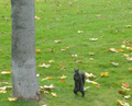
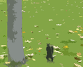
File:plane.jpg|Input RGB Image |
File:plane.jpg|Input RGB Image |
||
| − | File: |
+ | File:xu.15.prl-3063_map.png|Saliency map |
</gallery> |
</gallery> |
||
| − | |||
== Illustrations == |
== Illustrations == |
||
| + | === Saliency map computation on BSDS500 database === |
||
| − | === Natural image simplification with the Mumford-Shah functional optimized on the MToS === |
||
| + | |||
| − | The method minimizes the Mumford-Shah cartoon model constrained by the tree topology. It removes nodes from the tree until the energy doest not decrease anymore. |
||
| − | The |
+ | The first test was performed on the [http://www.eecs.berkeley.edu/Research/Projects/CS/vision/grouping/resources.html BSDS500] database. Some samples are given below and full results are available in this [https://lrde.epita.fr/~xu/material/saliency-maps-BSDS500.tar.gz archive]. The results are obtained |
| + | relying on the gradient image of Structured Edge. |
||
| + | |||
| + | <gallery caption="From top to bottom: input images; saliency maps; slight/moderate/strong simplification." perrow=5> |
||
| + | File:Xu.15.prl-100007.png |
||
| + | File:xu.15.prl-196027.png |
||
| + | File:xu.15.prl-8068.png |
||
| + | File:xu.15.prl-189080.png |
||
| + | File:xu.15.prl-3096.png |
||
| + | |||
| + | |||
| + | File:Xu.15.prl-100007_map.png |
||
| + | File:xu.15.prl-196027_map.png |
||
| + | File:xu.15.prl-8068_map.png |
||
| + | File:xu.15.prl-189080_map.png |
||
| + | File:xu.15.prl-3096_map.png |
||
| + | |||
| + | |||
| + | File:Xu.15.prl-100007_less_simp.png |
||
| + | File:xu.15.prl-196027_less_simp.png |
||
| + | File:xu.15.prl-8068_less_simp.png |
||
| + | File:xu.15.prl-189080_less_simp.png |
||
| + | File:xu.15.prl-3096_less_simp.png |
||
| + | |||
| + | |||
| + | File:Xu.15.prl-100007_median_simp.png |
||
| + | File:xu.15.prl-196027_median_simp.png |
||
| + | File:xu.15.prl-8068_median_simp.png |
||
| + | File:xu.15.prl-189080_median_simp.png |
||
| + | File:xu.15.prl-3096_median_simp.png |
||
| + | |||
| + | File:Xu.15.prl-100007_strong_simp.png |
||
| + | File:xu.15.prl-196027_strong_simp.png |
||
| + | File:xu.15.prl-8068_strong_simp.png |
||
| + | File:xu.15.prl-189080_strong_simp.png |
||
| + | File:xu.15.prl-3096_strong_simp.png |
||
| + | |||
| + | </gallery> |
||
| + | |||
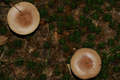
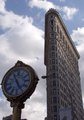
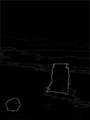
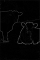
| + | === Saliency map computation on Weizmann database === |
||
| + | |||
| + | The second test was performed on the [http://www.wisdom.weizmann.ac.il/~vision/Seg_Evaluation_DB/ Weizmann] database. Some samples are given below and full results are available in this [https://lrde.epita.fr/~xu/material/saliency-maps-weizmann-2obj.tar.gz archive]. The results are obtained relying on the gradient image of Structured Edge. |
||
| + | |||
| + | <gallery caption="From top to bottom: input images; saliency maps; slight/moderate/strong simplification." perrow=5> |
||
| + | File:Xu.15.prl-109300481333.png |
||
| + | File:xu.15.prl-112224059330.png |
||
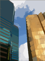
| + | File:xu.15.prl-kata.png |
||
| + | File:xu.15.prl-hotblack_20070901_cows.png |
||
| + | File:Carlinet.15.tip-p5014757_cropped.png |
||
| + | |||
| + | File:Xu.15.prl-109300481333_map.png |
||
| + | File:xu.15.prl-112224059330_map.png |
||
| + | File:xu.15.prl-kata_beach_phuket_map.png |
||
| + | File:xu.15.prl-hotblack_20070901_cows_map.png |
||
| + | File:xu.15.prl-p5014757_cropped_map.png |
||
| + | File:Xu.15.prl-109300481333_less_simp.png |
||
| − | <gallery caption="Top: original images. Bottom: simplified images." perrow=5> |
||
| − | File: |
+ | File:xu.15.prl-112224059330_less_simp.png |
| − | File: |
+ | File:xu.15.prl-kata_beach_phuket_less_simp.png |
| + | File:xu.15.prl-hotblack_20070901_cows_less_simp.png |
||
| − | File:carlinet.15.tip-B17paul1444.png |
||
| + | File:xu.15.prl-p5014757_cropped_less_simp.png |
||
| − | File:carlinet.15.tip-nopeeking.png |
||
| − | File:carlinet.15.tip-p5014757_cropped.png |
||
| − | File: |
+ | File:Xu.15.prl-109300481333_median_simp.png |
| − | File: |
+ | File:xu.15.prl-112224059330_median_simp.png |
| − | File: |
+ | File:xu.15.prl-kata_beach_phuket_median_simp.png |
| + | File:xu.15.prl-hotblack_20070901_cows_median_simp.png |
||
| − | File:carlinet.15.tip-nopeeking_simp.png |
||
| + | File:xu.15.prl-p5014757_cropped_median_simp.png |
||
| − | File:P5014757_cropped.png |
||
| + | File:Xu.15.prl-109300481333_strong_simp.png |
||
| + | File:xu.15.prl-112224059330_strong_simp.png |
||
| + | File:xu.15.prl-kata_beach_phuket_strong_simp.png |
||
| + | File:xu.15.prl-hotblack_20070901_cows_strong_simp.png |
||
| + | File:xu.15.prl-p5014757_cropped_strong_simp.png |
||
</gallery> |
</gallery> |
||
Latest revision as of 12:38, 10 March 2016
Materials
Mumford-Shah Simplification on the Color Tree of Shapes
You can download the x86_64 binary to compute the Mumford-Shah simplification running on the color tree of shapes Here.
Usage: ./mumford_shah_on_ctos input[rgb] α₀ α₁ λ output[rgb]
α₀	Grain filter size before merging trees (0 to disable)
α₁	Grain filter size on the color ToS (0 to disable)
λ	Mumford-shah regularisation weight (e.g. 5000)
Input RGB Image
Output Simplified Image

Input RGB Image

Output Simplified Image


Saliency Map Computation Relying on Mumford-Shah-Salient Level Line Selection
You can download the x86_64 binary to compute the saliency map representing hierarchical image simplification and segmentation Here. This application outputs the saliency map as a float image. The simplification and segmentation result can be obtained by thresholding this float image. Note that the image is twice as big as the original one and has a border for topogical and algorithmic purposes. Thus, any pixel with coordinates (x,y) in the original image is now at coordinates (2*(x+1), 2*(y+1)) in the saliency map.
Usage: ./saliency_map_mumford_ctos input[rgb] α₀ α₁ output[float]
α₀	Grain filter size before merging trees (0 to disable)
α₁	Grain filter size on the color ToS (0 to disable)
In the previous binary, we use the absolute difference between values of neighboring pixels to compute the average of gradient's magnitude, which is used to sort the shapes. An alternative is to use a gradient image given by a sophisticated contour detection method (e.g., the Structured Edge) to compute the average of gradient's magnitude. You can download this x86_64 binary Here.
Usage: ./saliency_map_mumford_ctos_grad input[rgb] α₀ α₁ gradSE.pgm output[float]
α₀	Grain filter size before merging trees (0 to disable)
α₁	Grain filter size on the color ToS (0 to disable)
gradSE 	Gradient image given by a contour detection method (Gpb or SE)
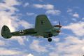
Input RGB Image

Saliency map


Illustrations
Saliency map computation on BSDS500 database
The first test was performed on the BSDS500 database. Some samples are given below and full results are available in this archive. The results are obtained relying on the gradient image of Structured Edge.
- From top to bottom: input images; saliency maps; slight/moderate/strong simplification.
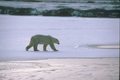


Saliency map computation on Weizmann database
The second test was performed on the Weizmann database. Some samples are given below and full results are available in this archive. The results are obtained relying on the gradient image of Structured Edge.
- From top to bottom: input images; saliency maps; slight/moderate/strong simplification.